




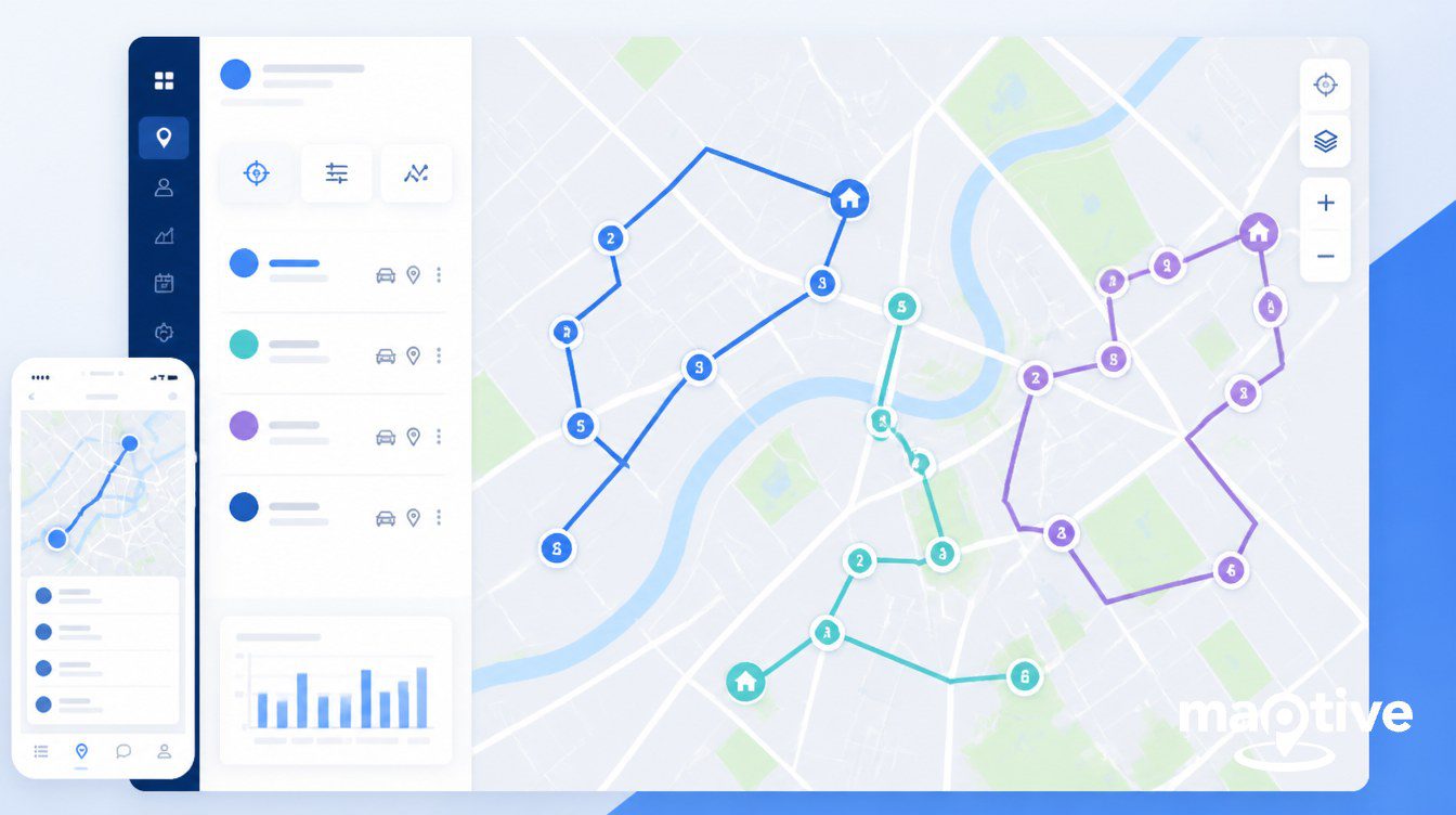
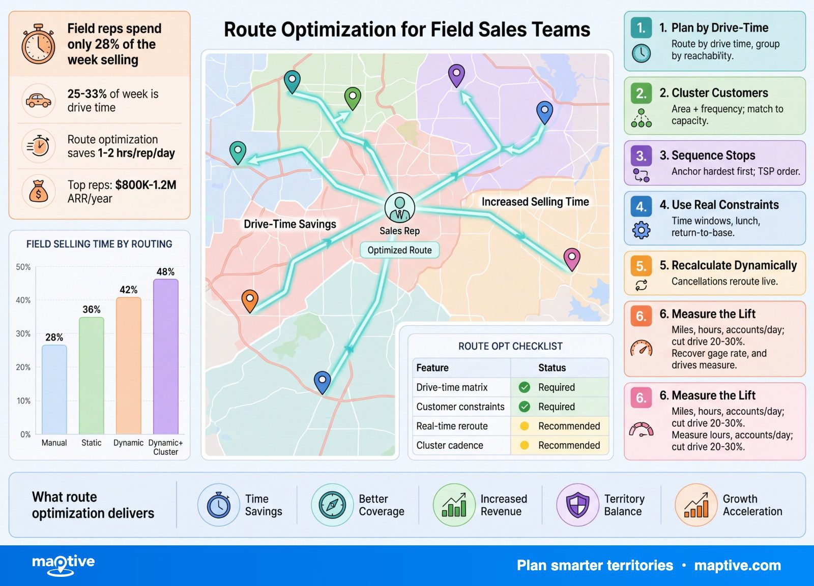
Route optimization for field sales is the practice of sequencing a rep’s daily or weekly visits to minimize drive time and cost while respecting appointment windows, account priority, vehicle and driver constraints, and live traffic. It applies the math of the Traveling Salesman Problem and the Vehicle Routing Problem to a real territory and a real CRM.
The pressure on this practice is plain. Outside sales reps average 21 hours per week behind the wheel, and 18% of reps report more than 40. Roughly 45% of an outside rep’s working time goes to traveling between client locations. Only 28% to 35% of the average sales rep’s week is spent actively selling. Every hour of drive time is an hour the rep cannot meet an account, log a call, or close a deal.
The math is also against the planner. A 10-stop day has more than 3.6 million possible orderings. A 50-stop route, brute forced, would take longer than the age of the universe to enumerate on current hardware. That is why production routing engines do not look for the perfect answer. They look for a very good answer fast, and the rest of this article covers how that decision shapes the way a field-sales team plans, executes, and measures its days.
The Routing Math Behind Field Sales
The TSP and VRP Foundations
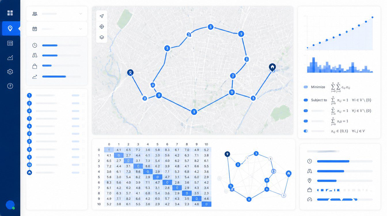
Two formal problems sit underneath every sales-route question. The first is the Traveling Salesman Problem, which asks for the shortest route that visits each of a list of locations exactly once and returns to the start. The second is the Vehicle Routing Problem, the multi-vehicle generalization of the TSP. Given a fleet of reps and a set of accounts, the VRP finds the optimal set of routes that serves every account at minimum total cost. Reduce the fleet to a single rep and the VRP collapses back into a TSP.
Both problems are NP-hard. The number of possible route orderings grows as the factorial of the stop count, which becomes intractable very quickly. A 10-stop tour has 10! orderings, or 3,628,800. A 30-stop tour produces a number with 32 digits. At a million permutations checked per second, brute forcing a 30-stop tour would require more than 200,000,000,000,000,000 years. A 57-stop route has roughly a 75-digit number of possible orderings. Brute force is not a strategy. It is an upper bound on what is possible to compute.
Heuristics and Metaheuristics in Production Solvers
Exact algorithms such as branch-and-bound and dynamic programming improve on brute force, but they still scale exponentially and become impractical past about 20 to 30 stops for repeated daily use. Production routing engines therefore rely on heuristics and metaheuristics. A heuristic gives up the guarantee of optimality in exchange for speed.
The simplest heuristic is nearest-neighbor. Start at a chosen depot, go to the closest unvisited stop, repeat. Nearest-neighbor is fast and easy to implement. It is also greedy and shortsighted, often locking in early choices that force long final legs. A human looking at the same map will frequently spot a shorter route.
Genetic algorithms treat candidate routes as a population that breeds and mutates across generations. Routes with shorter total distance survive into the next generation. With enough iterations, a genetic algorithm finds shorter routes than nearest-neighbor, although it still does not guarantee the global optimum. Hybrid methods improve further. A common approach for the Capacitated VRP uses a genetic algorithm to assign customers to vehicles and then a nearest-neighbor heuristic to sequence each vehicle’s route. The hybrid outperforms either method alone.
Google’s OR-Tools is the most widely cited open-source optimization toolkit for TSP and VRP. It combines local search with metaheuristics such as guided local search, simulated annealing, and tabu search. The pattern is consistent across commercial routing engines as well. Find a feasible starting solution, then move stops between routes and swap orderings under a guiding rule until the solution stops improving.
Isochrones, Time Matrices, and Multi-Depot Variants
Two supporting concepts appear repeatedly in routing workflows. An isochrone is a contour around a starting point that encloses every location reachable within a specified travel time, given current traffic and road network conditions. A 30-minute isochrone from a downtown office at 9 a.m. covers a different set of accounts than the same isochrone at 2 p.m., because congestion compresses or expands the reachable area. Planners use isochrones to test feasibility before sequencing. The second concept is the time matrix, a precomputed table of travel times between every pair of stops, sometimes updated multiple times per hour against live traffic data. The quality of the time matrix sets the upper bound on what any heuristic can achieve. A solver running on a stale or coarse matrix produces an elegant plan that breaks when the rep encounters real traffic. The practical implication for buyers of routing software is that the underlying map data, traffic feeds, and time-matrix refresh cadence matter as much as the algorithm name on the marketing page. A weaker heuristic on fresh data routinely beats a stronger heuristic on stale data.
Multi-depot variants raise the complexity again. Multi-Depot VRP (MDVRP) sits among the hardest classes of routing problem because the algorithm must first decide which depot serves which customer, then sequence each resulting route. Modern solvers handle 200-stop multi-depot routes in under 300 milliseconds and 500-stop multi-depot multi-period routes in roughly 3 seconds. Multi-day route optimization APIs allow up to 20 days of forward scheduling against 50 or more hard and soft constraints, including working hours, waiting time, task lateness, and vehicle capacity. The academic formulation for sales reps who do not return to a depot is the Multi-Depot Open VRP with Time Windows (MDOVRPTW). Open VRP relaxes the requirement to return to the start. Closed VRP enforces it.
The takeaway from the math is practical. Past about 15 stops, no field-sales planner is computing an optimum in their head, on a whiteboard, or in a spreadsheet. They are running a heuristic, with or without naming it that. Choosing a routing engine is largely a choice of which heuristics it implements and how well its constraint model captures the real workflow. A solver that produces a mathematically shorter route but ignores account tier or service duration produces a worse business outcome than a heuristic that respects both.
Variables and Constraints That Shape a Real Route
The Core Variables in a Sales Route Model
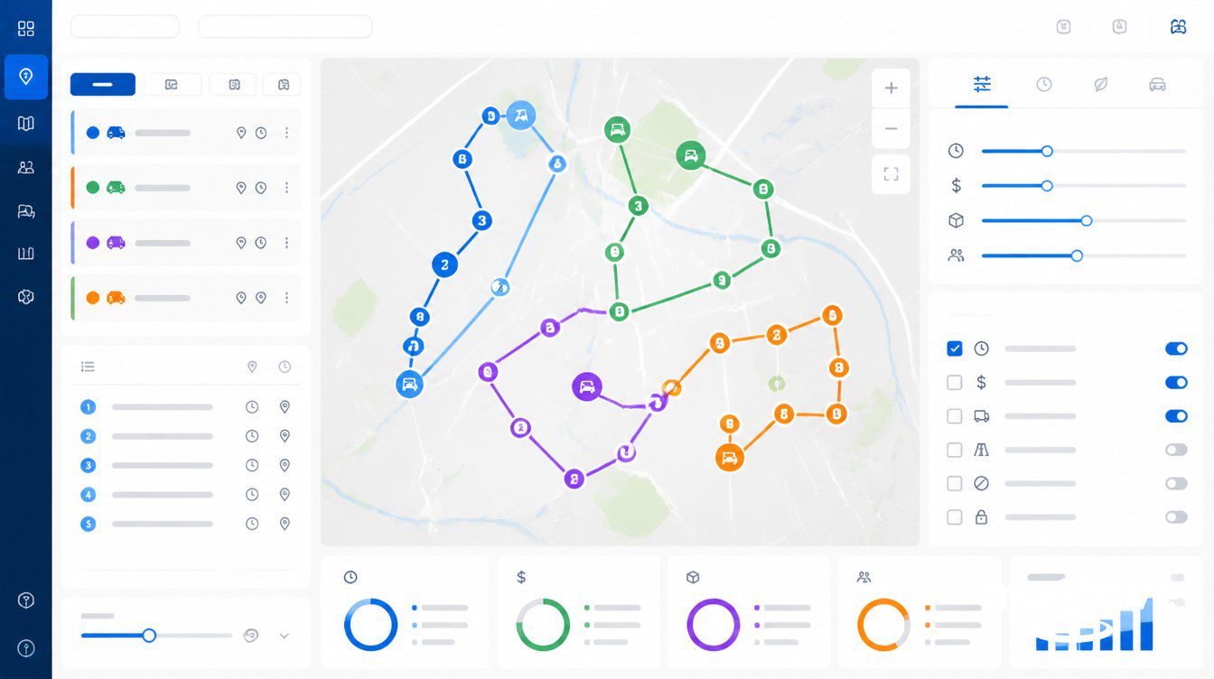
The textbook TSP optimizes one number, total distance. A real field-sales route optimizes against many constraints at once, and the relative weight of those constraints determines if a route is usable or only mathematically short.
The variables that matter for sales route optimization include the following.
Distance and live traffic. The straight-line distance between two stops is rarely the actual travel cost. Drive time at 7:45 a.m. is not drive time at 11:00 a.m. Routing engines that ignore traffic produce plans that fail by mid-morning.
Time windows. Most accounts can only be visited within a defined window, often dictated by clinic hours, store delivery windows, buyer calendars, or contractual appointments. A window of 8:00 a.m. to 10:00 a.m. is a hard constraint. A preferred window of afternoons is a soft one.
Account tier and visit cadence. A common framework assigns A, B, and C tiers. A accounts may be visited every two weeks, B monthly, C quarterly. An alternative model treats the top 20% of revenue accounts as Tier 1 with weekly or bi-weekly visits, the middle 30% to 40% as Tier 2 with less frequent contact, and the long tail as Tier 3.
Service duration per stop. A 5-minute drop-off and a 45-minute discovery meeting cannot be treated as equivalent. Service time per stop drives the difference between a day plan with 12 visits and one with 5.
Vehicle and driver capacity. Sample inventory, demo equipment, brochures, and physical goods all consume cargo space. Drivers have legal and contractual hour limits.
Depot and home anchoring. Some reps start at a regional office. Some start at home. Some end at home regardless of where the day began. The routing problem changes when the rep must return to the depot (closed VRP) versus ending the day wherever the last stop sits (open VRP).
Geocoding accuracy. A route is only as good as the coordinates underneath the addresses. CRMs accumulate dirty addresses over years of manual entry, and a single zip-code typo can send a rep across town.
Time Windows, Tiering, and Open Versus Closed VRP
Time windows deserve close attention because they are the constraint planners most often get wrong. Set a window too narrow and the route contains forced idle time, the rep arrives early and waits. Set the window too wide and the customer must keep themselves available longer than the actual visit needs. Both errors waste hours per week. The right window respects the customer’s actual calendar without padding it.
Account tiering is the second source of common error. The A/B/C model is a starting point, not a finished cadence. A territory’s revenue concentration determines how aggressive the Tier 1 cadence should be. A field rep covering 12 hospital systems with 80% revenue concentration in three of them will not produce useful plans if all 12 are treated as equal weekly stops.
Vehicle capacity and driver hours apply unevenly across field-sales verticals. A pharma rep in a sedan with a tote of samples has minimal capacity constraints. A medical device rep transporting a loaner instrument tray, or a beverage merchandiser servicing 30 to 50 stops on a beverage direct-store-delivery route, has capacity as a hard constraint.
Open VRP versus closed VRP sounds academic and turns out to be the routing concept most relevant to outside reps. An outside rep almost never returns to a warehouse. The day ends at home, at the last appointment, or wherever the rep parked. Modeling the route as open removes a phantom final leg that closed-VRP solvers force into the plan, and it is the difference between a route that reflects how the rep actually works and one that adds 45 minutes of fictional driving every evening.
Geocoding sits beneath everything else. A 2024 benchmark across major geocoding APIs found Google’s geocoder most reliable, with other providers less accurate on rural and non-U.S. addresses. No provider matches every address perfectly because typos, abbreviations, and incomplete CRM records cannot always be resolved. Address hygiene is therefore an upstream variable. The cleanest routing engine produces a broken plan if the addresses are wrong.
Vertical-Specific Constraint Patterns
The verticals where these constraints bite hardest illustrate the spread. A pharmaceutical rep operates against tight clinic windows, short call durations of 5 to 10 minutes, and access rates that have only recovered to roughly 60% of pre-pandemic levels in 2023 to 2024. The route must respect lunch closures, surgical block schedules, and the difference between an academic medical center and a community clinic. A medical device rep starts the morning at a scheduled surgical case and routinely loses the afternoon to trauma cases or after-hours surgeries, with the rest of the day bending around the unscheduled. A beverage direct-store-delivery driver runs a fixed weekly route of 30 to 50 stops across convenience stores, restaurants, grocery, and bars. The route is largely cyclical, with margin for substitution only when a store is closed for inventory or remodel. A B2B account executive in industrial distribution or building products has fewer stops, longer service durations, and more variability in appointment confirmation.
Each of these patterns implies a different default for the constraint model. The pharma rep needs tight time windows and short service durations weighted heavily. The medical device rep needs aggressive replanning logic and tolerance for high cancellation rates. The DSD driver needs a cyclical template that holds the base route stable. The B2B account executive needs strong tier weighting and looser windows.
Regulatory Constraints in Pharma Routing
Regulatory constraints also belong in the constraint model where they apply. The Drug Supply Chain Security Act requires real-time electronic interoperability and serialization to the package level across the U.S. pharma supply chain as of November 24, 2024. Civil fines can reach $500,000 per violation, and intentional violations may produce criminal charges. Field-based pharma reps handling samples must follow the serialization workflow at every transfer, which means the routing engine has to account for sample-handling stops, secure storage requirements, and electronic signature steps as part of service duration.
Static Routes, Dynamic Routes, and the Replanning Trigger
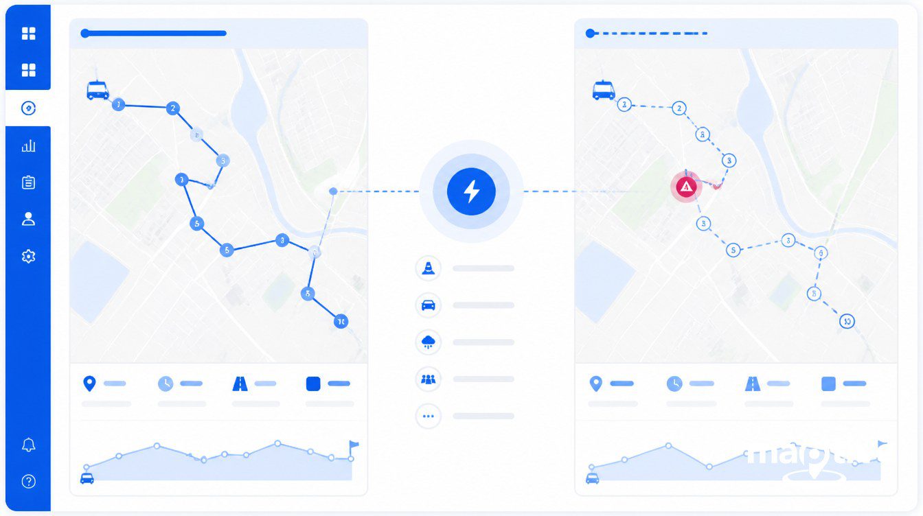
The next decision is between a route computed once and followed and a route computed continuously and adjusted as conditions change. The first model is static routing. The second is dynamic routing. Both have legitimate use cases in field sales, and the choice depends on how much of the day is fixed when the rep leaves the house.
Static routing computes a plan in advance, usually the night before or the morning of, and the rep follows it as written. A static plan is appropriate when accounts have predictable cadences, appointments are confirmed, traffic is regular, and cancellations are uncommon. Many pharma territories and most beverage DSD routes run on a static base schedule that varies only at the margins. Static routes also serve compliance because the plan can be archived, audited, and compared against actual driving history.
Dynamic routing replans in real time. When a customer cancels, a meeting runs long, a new urgent visit appears, traffic shuts a corridor, or a high-priority lead comes in mid-morning, the routing engine recomputes the remaining stops and pushes the updated sequence to the rep’s device. AI routing agents monitor live feeds and trigger replanning when defined thresholds are breached.
The market data shows where the investment is going. The global dynamic route optimization software market was estimated at $1.9 billion in 2024 and is forecast to reach $6.6 billion by 2034. The wider route optimization market was $10.99 billion in 2025 and is projected at $42.65 billion by 2035. Last-mile delivery dominates the dynamic segment with roughly 33% market share. Field sales is a smaller but faster-growing slice driven by AI-enabled CRMs.
Predictive ETAs are the visible output of the dynamic stack. Machine-learning models trained on traffic patterns, weather, vehicle telemetry, and historical performance now predict arrival times with 90% to 95% accuracy. For field sales, this matters because it lets the rep give an account a tight ETA window instead of a 30-minute fudge.
When Static Routing Holds Up
Static routing is the right choice when three conditions are present. The accounts on the list have agreed appointment times or fall inside predictable windows. The territory geography is stable. The rep’s day rarely changes mid-morning. Many enterprise and named-account territories fit this profile.
The advantage of static routing is auditability and discipline. A plan that is set the night before forces tier discipline. A plan that recomputes every 20 minutes can hide drift, the slow replacement of A accounts with closer-but-lower-tier B and C accounts.
When Dynamic Replanning Pays For Itself
Dynamic routing earns its keep in territories where the day breaks. A medical-device rep who starts every morning at a scheduled surgical case will frequently end up in an after-hours trauma case the same day. A beverage merchandiser who finds a store closed for inventory will lose the visit unless the engine reslots the stop.
The replanning trigger is the operationally meaningful concept here. A dynamic engine should not replan continuously, because that destroys the rep’s ability to commit to ETAs. It should replan when a defined threshold is crossed.
A useful field test of the case for dynamic routing in a given territory is the cancellation rate. If less than 5% of stops cancel or move on the day, static routing with daily replanning at 6 a.m. or 7 a.m. is enough. If 15% or more of stops change between morning and afternoon, the rep is replanning manually all day, and dynamic routing recaptures that lost time.
The Daily Planning Workflow as Reps Actually Run It
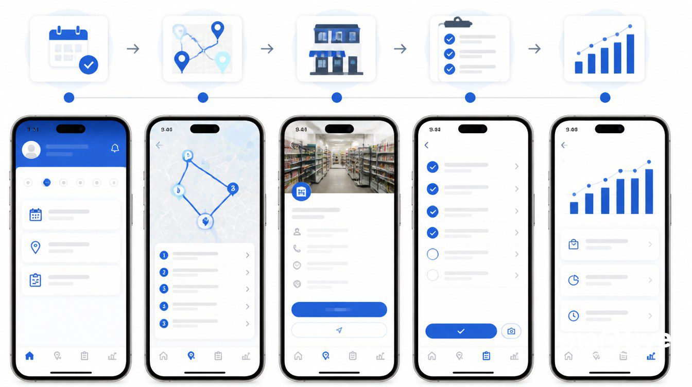
The Six-Step Day-Plan Sequence
The mechanics of a day plan have stabilized into a six-step workflow that recurs across verticals. CRM pull, priority and tier sort, route compute, calendar sync, mobile dispatch, activity logging.
Each step has a failure mode. CRM pulls fail when the underlying CRM data is stale. Tier sorts fail when the tier definitions have not been reviewed in 12 months and no longer match revenue concentration. Route computes fail when constraint settings are wrong. Calendar syncs fail when travel-time blocks are not included. Mobile dispatch fails when the rep ignores it in favor of a consumer navigation app. Activity logging fails when the friction of logging is high enough that reps batch it at the end of the week.
CRM Integration and the Limits of Consumer Maps
Consumer mapping tools cannot stand in for this workflow at any meaningful scale. Google Maps allows a maximum of 10 destinations per route, will not automatically reorder them for efficiency, and cannot push real-time changes back to a planner. A rep doing 15 to 25 visits a day cannot manage that volume on a consumer maps app without juggling multiple maps or losing data when stops change.
Execution-State Friction and the Activity-Logging Loop
The activity-logging step at the end of the workflow is the one that operations teams undervalue most. A logged stop produces three pieces of data that the next day’s plan depends on. The actual arrival and departure times, which calibrate service duration estimates. The visit outcome, which adjusts tier and cadence. Any rep notes about access or scheduling, which update the constraint model for the next visit. Reps who batch-log at the end of the week destroy this loop.
Common Failure Modes in Sales Route Planning
Routes break in predictable ways. Planning by zip code alone, ignoring time windows, no buffer time, weekly plans where daily replanning is needed, quantity of stops over account value, relying on driver memory, and dirty CRM addresses are the most common failures.
Address Hygiene and Geocoding Failure
Address quality is the upstream cost driver that most teams underinvest in. A single wrong zip code in a CRM can send a rep across town to a wrong address, costing 30 to 60 minutes per occurrence and one missed visit. A field-sales operation with 100 reps and a 2% bad-address rate is losing roughly two rep-hours per day to address failures, which compounds to about 500 lost rep-hours per year across the team.
The Quantity-Over-Quality Trap
A second persistent failure mode is optimizing for stops per day as a primary metric. Stop count is easy to measure. Account value per stop is harder. The natural drift is to fill the day with closer, easier B and C accounts and let A accounts slide. The fix is to bake account tier into the routing constraint, not into a separate manual review step.
Measuring ROI on Route Optimization
Reported Savings and Per-Call Economics
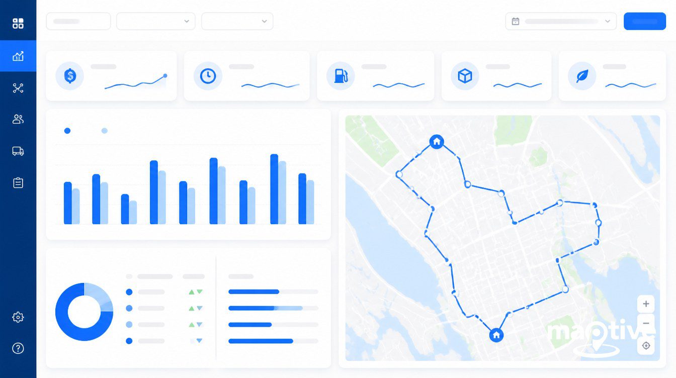
Reported savings from optimized routing fall in consistent ranges. Drive time and fuel drop by 20% to 40%. Miles driven fall by 10% to 15%. Total delivery and visit cost falls by 15% to 20%. Daily client visits increase by 18% to 44%, with an average of 3 to 5 additional visits per rep per day after adoption. Reps using routing software save roughly 8 hours per week on planning. Most companies see positive ROI within 3 to 6 months.
Translating those ranges into dollars requires the per-call cost. The average cost of an outside sales call is $215 to $400, compared with roughly $50 for an inside call. The IRS standard business mileage rate is 72.5 cents per mile in 2026.
A Worked ROI Calculation for a Five-Rep Team
For a 5-rep team: 30 minutes per rep per day saved on planning and driving, 5 reps, 240 working days per year equals 600 rep-hours per year. 3 additional visits per rep per day across 5 reps and 240 days is 3,600 additional visits per year, worth around $1.08 million in selling capacity at $300 per call. A 15% mile reduction on 100-mile-per-day across 5 reps saves 18,000 miles and $13,050 in direct cost. Fuel savings around $2,700. Planning time recovered: 2,000 hours per year.
Telematics, Override Data, and Fleet Composition
The ROI case strengthens further when paired with telematics. Fleet telematics separates productive idle time from waste idle, surfaces speeding and harsh braking, and feeds driver scorecards that managers can use in coaching. The argument against route optimization investment is almost always cultural rather than economic.
Rep Retention as the Compounding Driver
The largest single ROI driver is the compounding effect on rep retention. Average annual sales turnover sits at roughly 35%, three times the cross-industry average, and the all-in cost to replace a field rep is roughly $115,000 in recruiting, training, ramp, and lost opportunity. A retention improvement of even three to five percentage points on a 35% baseline, across a 20-rep team, recovers more than $200,000 in replacement cost per year.
Frequently Asked Questions
What is route optimization?
Route optimization is the process of finding the most efficient sequence of stops for one or more vehicles, factoring in distance, traffic, time windows, vehicle capacity, and stop priority. It is the practical application of the Vehicle Routing Problem and the Traveling Salesman Problem.
What is the Traveling Salesman Problem?
The Traveling Salesman Problem asks for the shortest route that visits every required location exactly once and returns to the start. It is NP-hard. With only 30 cities, exhaustively checking every possible route at a million combinations per second would take longer than 200 quadrillion years.
What is the Vehicle Routing Problem?
The Vehicle Routing Problem is the multi-vehicle version of the Traveling Salesman Problem. Given a fleet and a set of customers, it finds the optimal set of routes that serves every customer at minimum total cost.
How much time do sales reps spend driving?
Outside sales reps average 21 hours per week behind the wheel, with 18% of reps reporting more than 40 hours weekly. Roughly 45% of an outside rep’s working time goes to traveling between client locations.
How many sales calls per day should an outside sales rep make?
The average outside sales rep completes 5.1 in-person visits per day, or about 25 per week. Top performers average 8 to 12 face-to-face visits per day.
What is the IRS mileage rate for 2026?
The IRS standard mileage rate for business use is 72.5 cents per mile in 2026, up 2.5 cents from 70 cents per mile in 2025.
Can Google Maps optimize a sales route?
Google Maps allows up to 10 destinations per route, does not automatically reorder them for efficiency, and cannot push real-time changes back to a planner. A rep with 15 to 25 daily visits cannot manage that volume on a consumer maps app.
What is windshield time?
Windshield time is industry shorthand for the hours a field worker spends driving between appointments. Route optimization targets windshield time directly by sequencing stops to minimize between-visit travel.