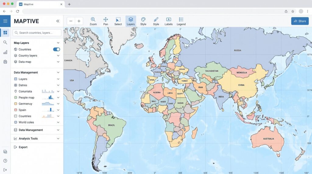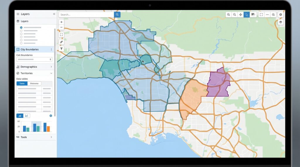



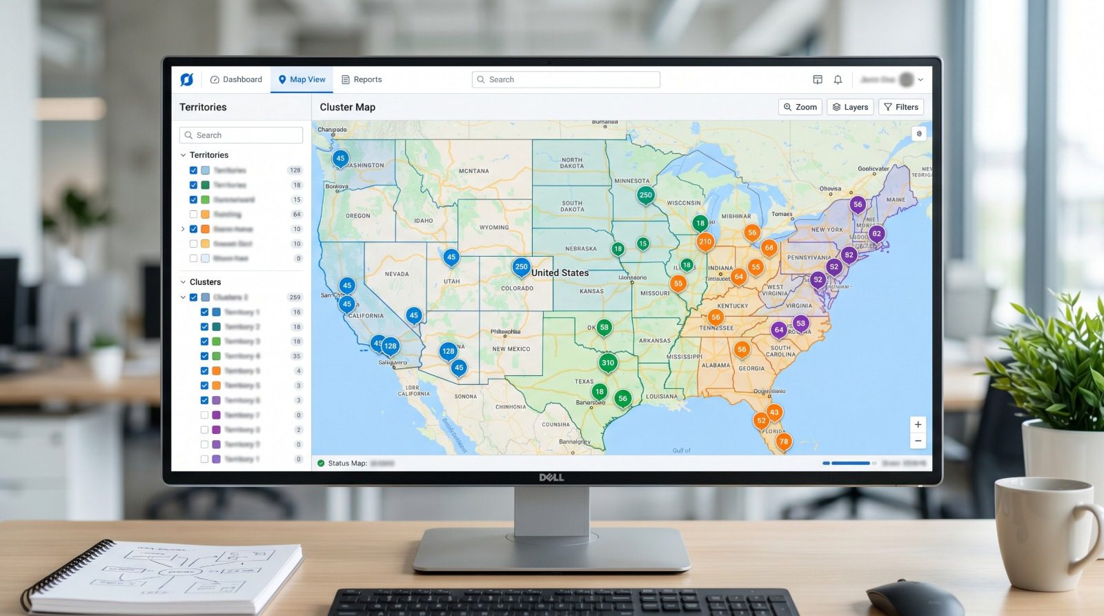
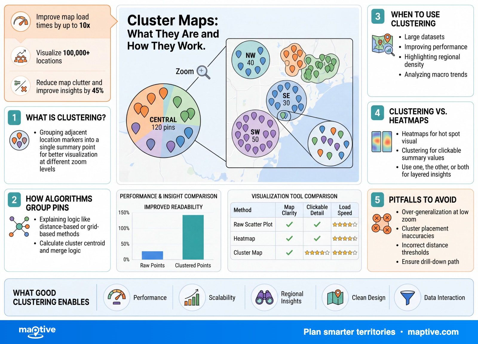
A cluster map groups nearby point markers into a single counted icon when they sit too close to show individually, and zooming in breaks it into smaller groups and finally the markers underneath. The number on the icon is the count of points it holds at the current zoom.
Picture two regions on a map, each a solid mass of overlapping dots. Turn clustering on and one reads 412, the other 207. Your eye cannot count piled-up dots, but it reads two numbers in a second, which is all a cluster map is built to do.
Cluster vs Choropleth: Points, Not Regions
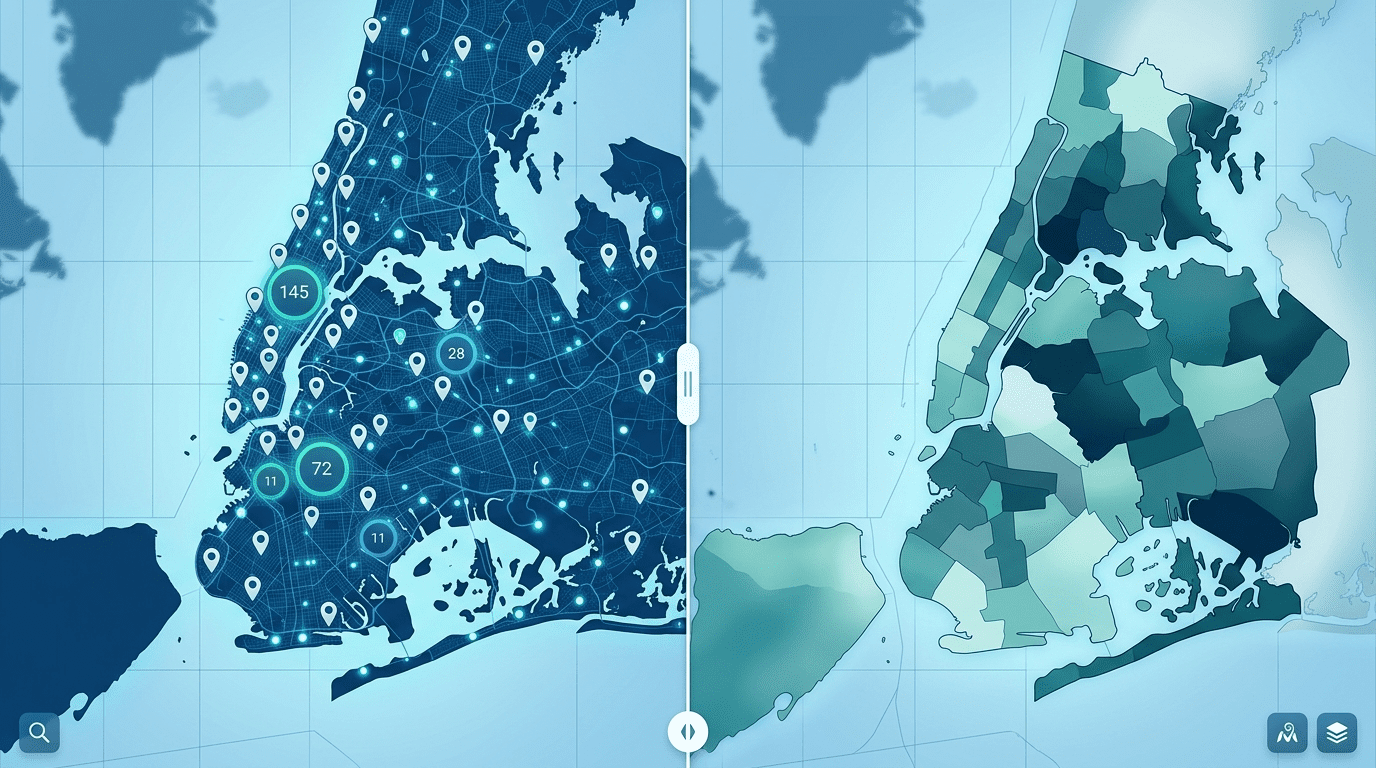
At its simplest, a cluster map takes a set of point markers that overlap into an unreadable blob and replaces the blob with a few counted icons. The points might be customer addresses, store locations, field assets, or accounts. When hundreds or thousands of them sit close together, individual pins disappear behind one another and the map stops telling you anything. Clustering hands the legibility back by collapsing the crowd into icons you can read, each with its count.
You will meet the same idea under several names. Marker clustering, point clustering, and bubble map all describe it, and the cluster icons are often called bubbles because they grow larger as their count grows. The one thing worth fixing early is what a cluster map is not. It works on individual points and the count of points in a screen neighborhood, with no predefined regions. A choropleth instead shades whole areas like states or ZIP codes by a value. Reach for clustering when the unit you care about is the point or the record, not the region.
The Mechanics of Marker Clustering
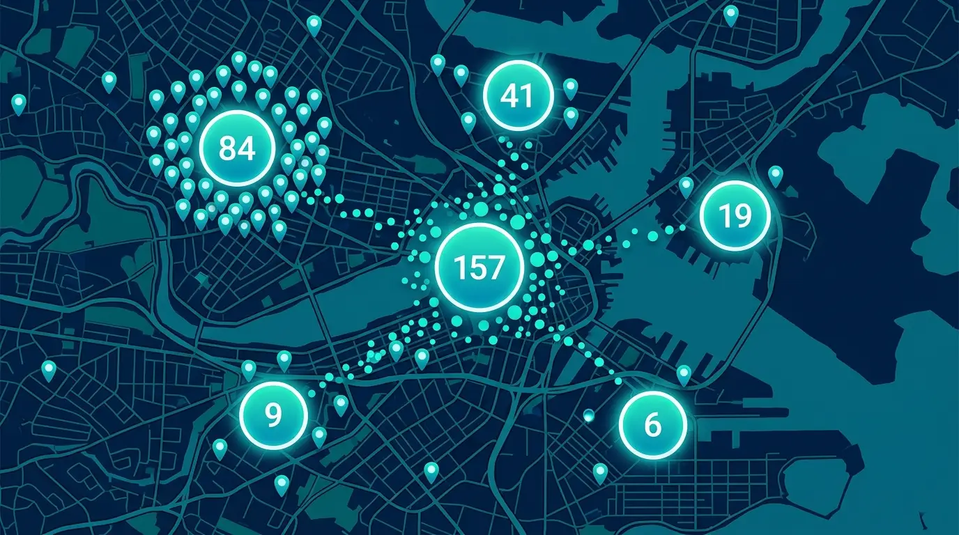
The easiest way to picture the mechanic is a grid laid over the screen. The map divides the visible area into cells, 60 by 60 pixels each. The first marker dropped into a cell becomes the seed of that cell’s cluster, every nearby marker that lands in the cell joins it, and the cluster’s icon moves to the average position of all its members. A marker that could belong to two clusters joins the nearer one.
One detail in that description does almost all the work, and it is worth slowing down on. The grid is measured in screen pixels, not in miles on the ground. Markers are grouped by how close they look at the current zoom, not by a fixed real-world distance. That single fact explains the behavior that surprises people most, since the same dataset clusters differently at every zoom level as the cells cover less ground.
Beyond the simple grid, mapping tools use a few different methods to do the same grouping. Distance-based approaches group points within a set radius of one another, and spatial-index methods speed the whole thing up on large datasets and avoid the flicker the older grid showed as the view changed. What these methods share matters more than how they differ, since every one of them groups nearby points and shows you a count. Most tools also expose a handful of controls worth knowing:
Grid or cluster size, which sets how aggressively points merge.
A maximum zoom past which clusters always break into individual markers.
A click-to-zoom option that fits the map to a cluster’s contents.
Reading the Number in the Bubble
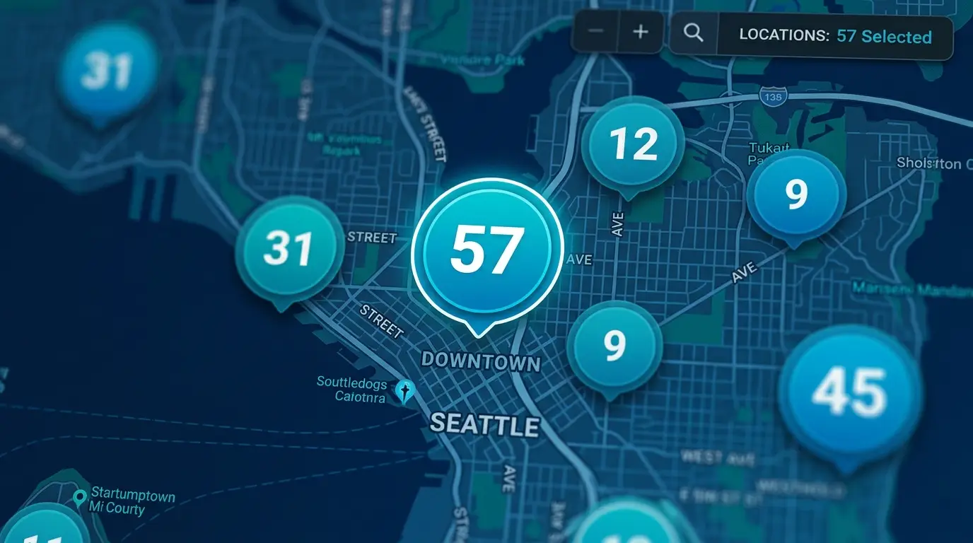
Read each bubble as “this many points are nearby at this zoom,” with a larger bubble meaning more points underneath. Clicking a cluster, or zooming in, breaks it open into the smaller clusters or the individual records it held. That much is intuitive once you have done it a few times.
A cluster can show more than a head count, which is where it earns real analytical reach. Instead of counting markers, it can show the sum of a value attached to each one, so a cluster of accounts can display combined sales for the group rather than only how many accounts there are, and the sub-clusters show the sum for their subset as you zoom in. It can also render as a live pie chart, breaking down the mix inside the cluster, such as which sales rep accounts for what share of a territory’s points. The bubble stops being a tally and becomes a small readout of whatever metric you fed it.
Here is the part to hold onto, because it is the most common way a cluster map gets misread. The count is a visualization aid. It tells you how many markers fall in a screen neighborhood at this zoom, and nothing more. An analyst who reads 318 on a cluster, screenshots it as the regional account total for a deck, then pans the map and watches the same points regroup into 204 and 151 has been caught by exactly this. The number was always tied to the zoom. The cluster’s icon adds a second wrinkle, since it floats at the averaged center of its members, which means it can sit where no actual marker is, and two clusters both labeled 20 can stand for very differently spread point sets. Read the count as a cue, then drill in before you draw a conclusion from it.
When to Cluster, When to Heat-Map, and When to Do Neither
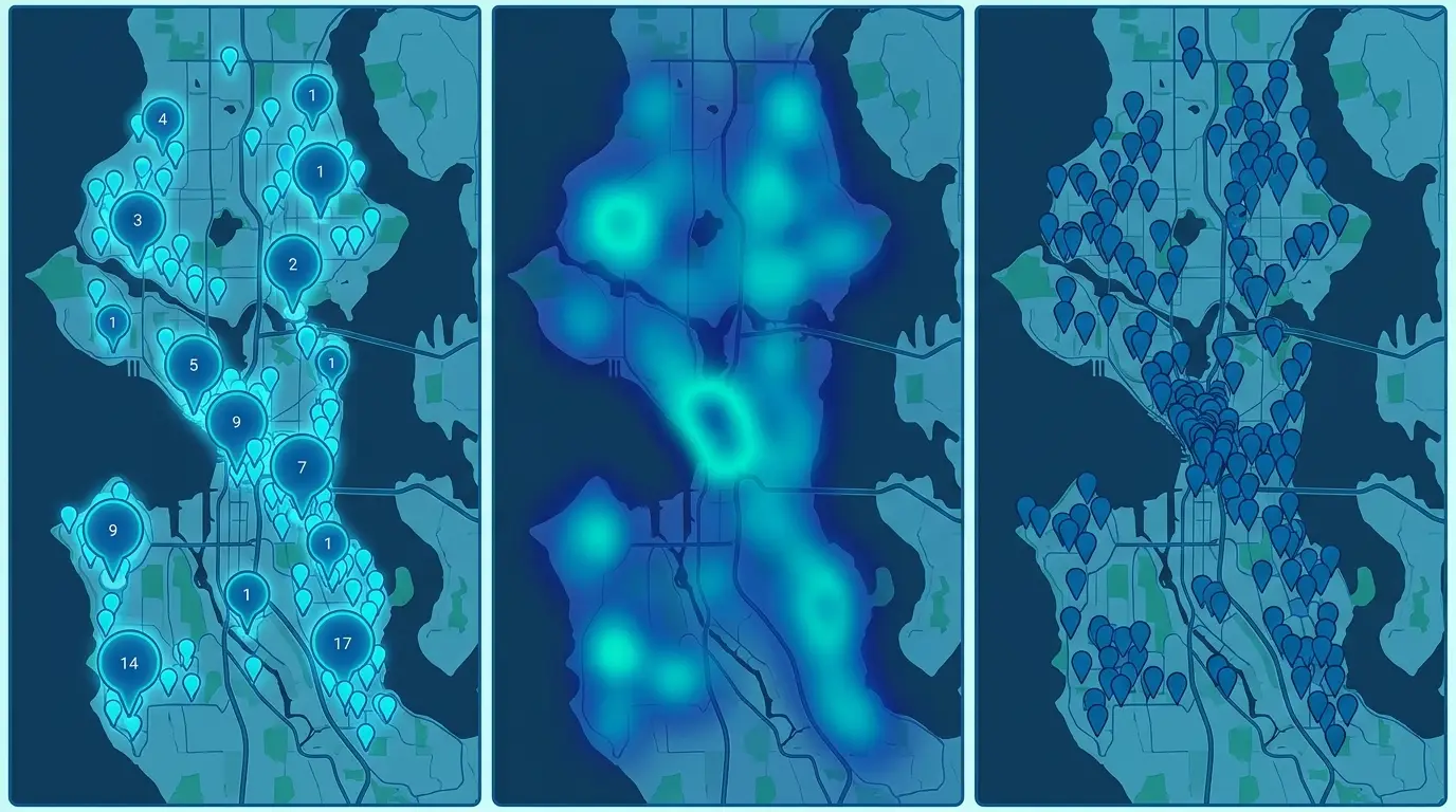
Clustering is one way to handle dense points, and a heat map is the other, and they answer different questions. The choice is less about which is better and more about what you are trying to see.
Cluster for Counts and Drill-Down
Cluster when you need to keep the count and the ability to click through to the individual records. This is the right tool when your data is point markers, the markers overlap into something unreadable, and you still want to know how many sit in an area and reach the records behind them. The cluster preserves a discrete, countable number and a path down to the underlying rows, which a smooth density surface gives up.
Heat-Map for Density at a Glance
Switch to a heat map when the question is about intensity rather than exact counts. A heat map renders a continuous color gradient, hot to cold, and conveys relative density without giving you a number to click into. It suits the case where points overlap so heavily that even clusters get crowded, or where you only need to spot the hot and cold zones at a glance. As a rough rule, heat maps read best when you are zoomed out and points pile up, while clustered or individual markers become more useful as you zoom in and the points separate.
There is a third answer that often gets missed, which is to use neither. Clustering is built to find groups, so it pushes isolated points into the background as leftover clutter. If your real job is to catch the lone account 200 miles from everything else, or the one underserved zone, clustering can bury the very signal you came to find. When the outlier is the point, plot the raw markers and let the isolated one show plainly.
The Case Against Clustering
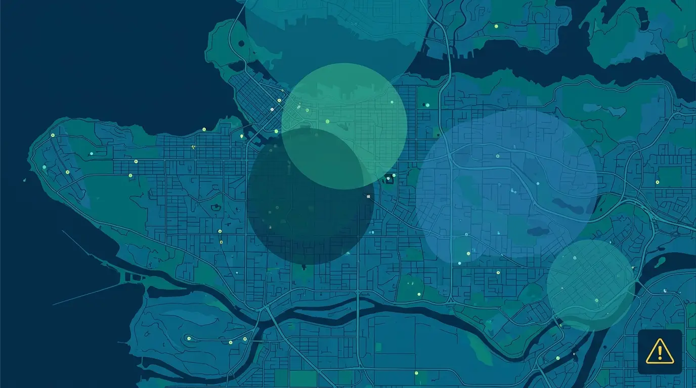
It is worth taking the strongest case against clustering seriously, because parts of it are right. A cluster sitting next to ordinary markers tells you nothing on its own. You have to click it or zoom to find out what is inside, so it answers a question with a question. Points at the same address can stay a closed box no matter how far you zoom, since zooming cannot separate markers that share coordinates. A screen covered in numbered bubbles is its own kind of cognitive load, not obviously less than a busy field of dots. And the original reason clustering existed, that older browsers choked on thousands of individual markers, has faded as modern map engines render large point sets quickly.
Each of those objections holds, which is why performance is no longer the main argument for clustering. A map dense with digits can be a strain to read. And co-located points do need a separate fix, called spiderfying, which fans markers at an identical address out into a small circle or spiral so each one becomes clickable once a cluster opens at high zoom.
What survives the objection is readability at the scale operations teams really work at. A sales or service dataset is rarely a few dozen points. It is thousands of accounts, or tens of thousands plotted on a single map, and at that volume a raw dump of markers is the unreadable blob the two-region example started with. Clustering turns it back into something you can compare and drill into, and the sum or pie-chart cluster encodes a metric a plain marker cannot. So the sensible call is to use clustering for what it does well and to reach for something else when it does not fit. Cluster to declutter an overlapping point set and preview where the weight sits, drill into the records when you need a real total, and leave clustering off when the lone point is the one you are hunting for.