



A US state map is one row of data for each state, shaded so that darker areas mean higher values. The first surprise arrives before any color does.
The same file of states can show up with 50 rows, 51, or 56, and which number you are looking at changes what the finished map is even claiming to show. The work that decides if it tells the truth happens in the table behind it and in two choices most people never stop to make.
Building the One-Row-Per-State Table

A state map reads one value for each state, so the build starts by collapsing your records down to that grain. If your spreadsheet holds one row per customer or one row per order, you sum or count those rows up to the state they belong to, and you end with exactly one row per state. The color the platform paints on Texas comes from that single Texas row, not the thousands of orders behind it.
This step is where most state maps are won or lost, and it gets skipped because the raw export looks map-ready already. It has a state column and a value column, so people upload it as is and let the tool figure out the rest. The tool then either errors or, worse, returns a finished-looking map that has summed the duplicate rows the wrong way without flagging it. Doing the aggregation yourself, in a pivot table before you map, means you know what each state’s number represents and you can sanity-check a few of the totals against what you already know about the business.
One fork is worth naming as you aggregate, because it sets up everything the color does later. A raw total answers a literal question, such as how much revenue you booked in a given state. A rate answers a comparative one, such as how deeply you have penetrated each state relative to its size, expressed as customers per 100,000 residents or revenue per account. If you are comparing states against one another, the rate keeps the comparison fair. If you only need the booked total, the raw number is the one you want. Decide which question the map is for before you reach for the shading.
Matching Rows to State Boundaries
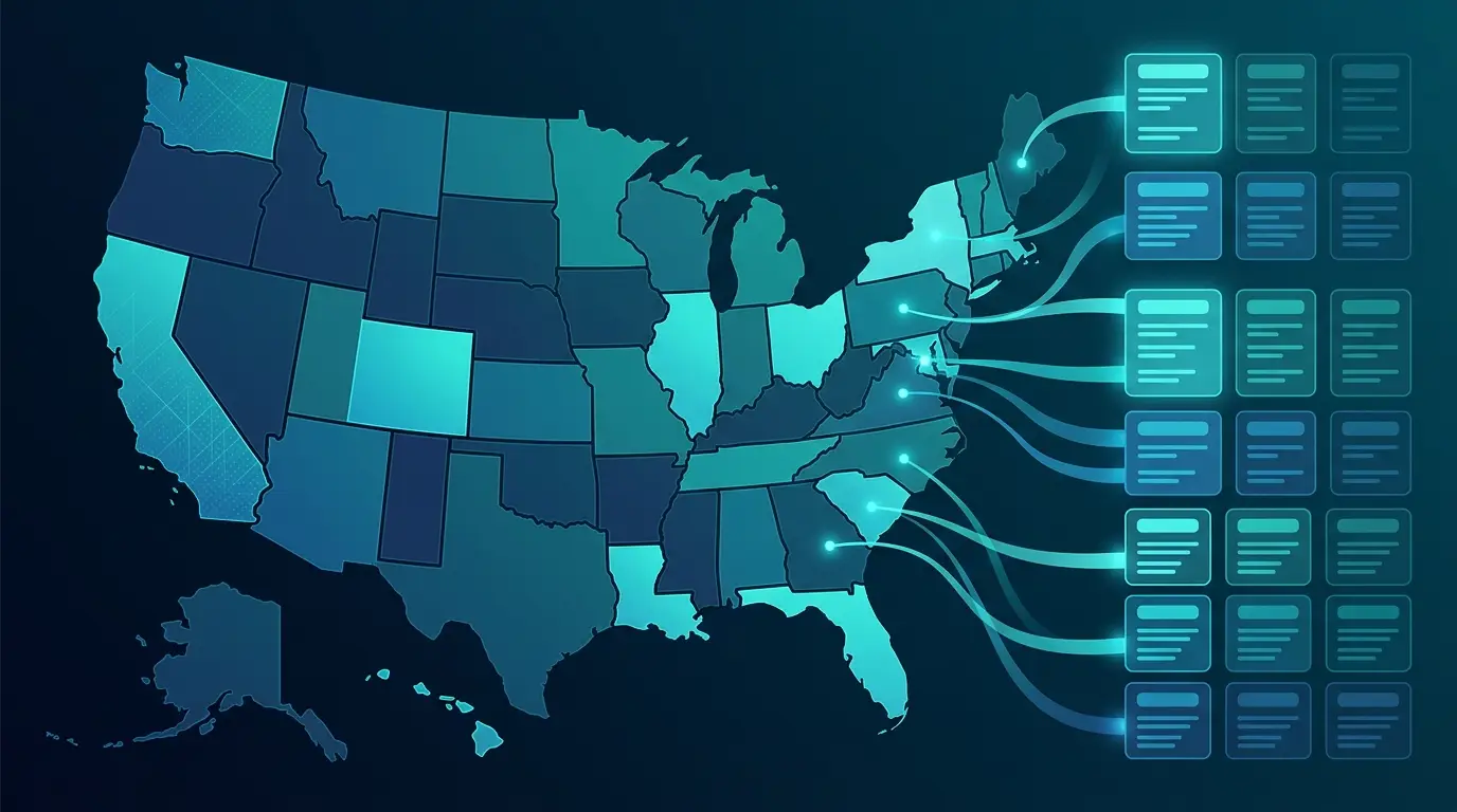
Once the table is at one row per state, the map needs to attach each row to the right shape on the map. Tools match on one of three keys, the full state name, the two-letter postal abbreviation, or the numeric FIPS code. The geometry almost never fails, so when a dozen states stay blank the key is what did not line up, not the map.
The classic failure is a half-gray map where a dozen states refuse to fill, and the cause is a key that does not line up. Some rows say “CA” and others say “California.” A trailing space hides at the end of a name. “Washington” the state gets confused with Washington as a stand-in for the capital. Spreadsheet map charts compound this, since some are limited to a single geography level and have been reported to recognize only 78% of states without an extra column to disambiguate them. The fix is to standardize on one key for every row and review the tool’s match table before you publish, so a pile of unmatched rows stops you rather than goes out with you.
What catches analysts off guard is that the dirty key usually started upstream. The same inconsistency that breaks the map also breaks syncs between systems, so the mix of abbreviations and full names was likely sitting in the CRM long before the data reached the map. You often repair the map by going back into the source records and cleaning the state field at its origin.
The Right Number of Rows on the Map

There are 50 states, so a US map almost always means 50 shapes. The District of Columbia is the wrinkle. It is a federal district built to hold the capital, so it is not a state and not a territory, yet most mapping tools fold it into their states geography anyway because analysts have data for it. That gives 51 areas. Add the five inhabited territories and you reach 56. State FIPS codes run from 01 up to 78 to make room for all of them.
So the row count is something you choose, since the same set of states can legitimately render as 50, 51, or 56 depending on what you include. If the business has records in Puerto Rico or the other territories, choose a states-and-territories geography that can render them, or roll those records into a separate bucket that stays off the map. One thing to avoid is enlarging or spotlighting the District of Columbia to make it visible, unless the map is specifically about it, since blowing up a tiny area distorts the read.
The Land-Area Bias in State Choropleths
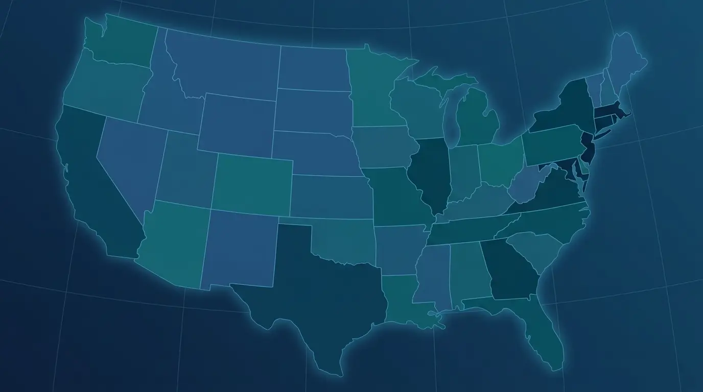
Here is the structural catch that no amount of clean data fixes on its own. A state choropleth gives every state a visual weight set by its land area, not by the value you are mapping. Large, sparsely settled states command the eye, and dense, productive states recede, regardless of what the numbers say.
The Montana-New Jersey Problem
Montana covers roughly 380,000 square kilometers and is home to about a million people. New Jersey covers roughly 22,000 square kilometers and holds about nine million. On a shaded map, Montana fills a wide block of the screen while New Jersey is small enough to overlook, even though New Jersey has nine times the population and, for most businesses, far more of the revenue. A handful of big-acreage, low-population states can visually swamp the dense coastal states where your accounts concentrate. This is the same effect that makes national election maps look lopsided, with sparse rural states painting large blocks of color and crowded metros barely registering.
When to Reach for a Bubble Map or Tile Cartogram
When that distortion would mislead the people reading the map, the choropleth is the wrong form for the job and there are two reliable replacements. A bubble map, also called a proportional-symbol map, places a circle on each state sized to its value, so a small state with a big number gets a big circle and area stops doing the talking. A hexagon tile cartogram replaces each state with a tile of identical size, which gives every state equal footing and removes land area from the picture entirely. Reach for one of these whenever the absolute counts matter and a few large states would otherwise drown out the rest.
Cutting the Color Into Bands
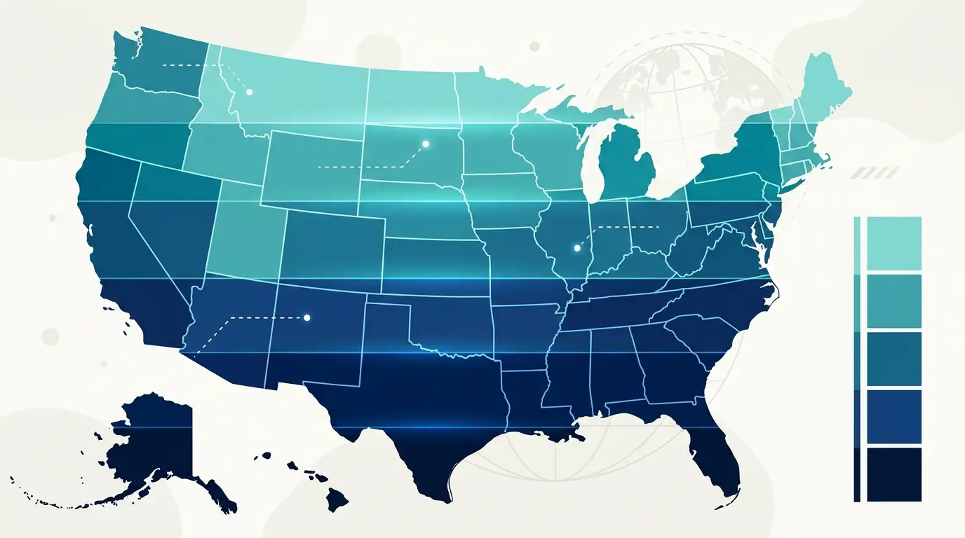
The number of shades and where you draw the lines between them is an editorial choice, and switching it can rearrange which states look high without a single number changing. The honest move for state data is to put the breaks where the values genuinely cluster, because business numbers across 50 states are almost always skewed, with a few large states and a long tail, and even-width bands will pile most of the map into one shade and waste the rest. Where exactly to cut, and how the named approaches trade off, is covered in depth in the choropleth guide. For a state map the practical test is simple, that two states a stakeholder would call clearly different should not land in the same band.
Hold the count between three and seven bands, since readers struggle to tell more shades apart than that, and use a single-hue scale that runs light to dark for ordered values like sales. Save a two-hue diverging scale for metrics that fall above or below a meaningful midpoint, such as growth against decline. The point that saves you a misread later is consistency. If you build a map for this year beside one for last year, keep the classification identical across both, or the comparison lies even though both maps look right. Two more habits keep the shading readable. Build the steps from distinct levels of lightness rather than from hue alone, since two states sitting in nearly the same shade can differ by a third in their underlying numbers and a stakeholder will read them as equal. Then preview the map in grayscale and against a color-vision-deficiency simulation, and avoid pairing red with green, so the map survives the screens and the eyes it will meet.
Rolling States Up to Regions
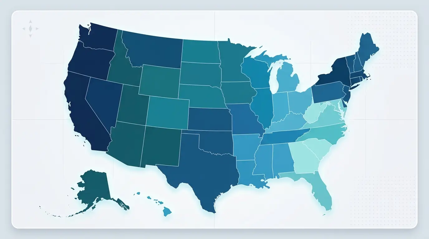
Reporting rarely stops at 50 states. It rolls them into regions or divisions, and a state map can show that in one of two ways. You add a region field to the data and color by region, or you keep the state shading and draw region outlines on top of it. Either reads cleanly, and the choice depends on if leadership wants to see the region as the unit or the states inside it.
The math at the region level is where this goes wrong without anyone noticing, and it is easy to miss. When you roll a rate up to a region, you cannot average the state rates together. A region’s true rate comes from its own summed numerator over its own summed denominator, such as total regional customers over total regional population. Raw counts add up without trouble, but rates do not, and a region figure built by averaging will look fine on the map while being wrong underneath. The same discipline that earned you a defensible state map applies at the region level, and the land-area bias from earlier applies here too, so reach for bubbles or equal-size tiles when the absolute counts are the point.
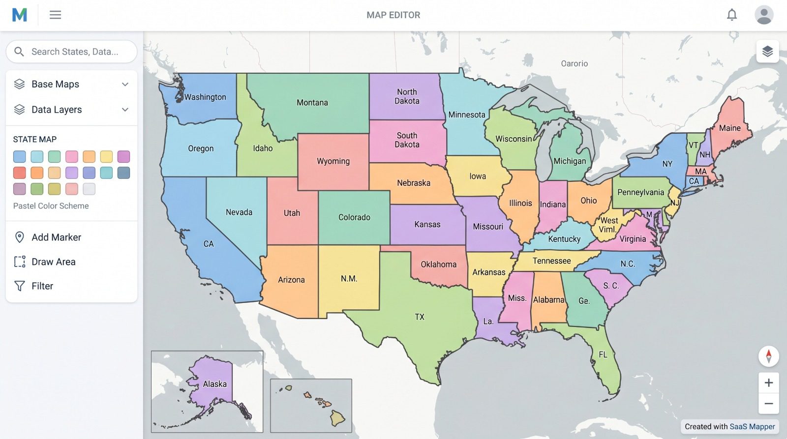
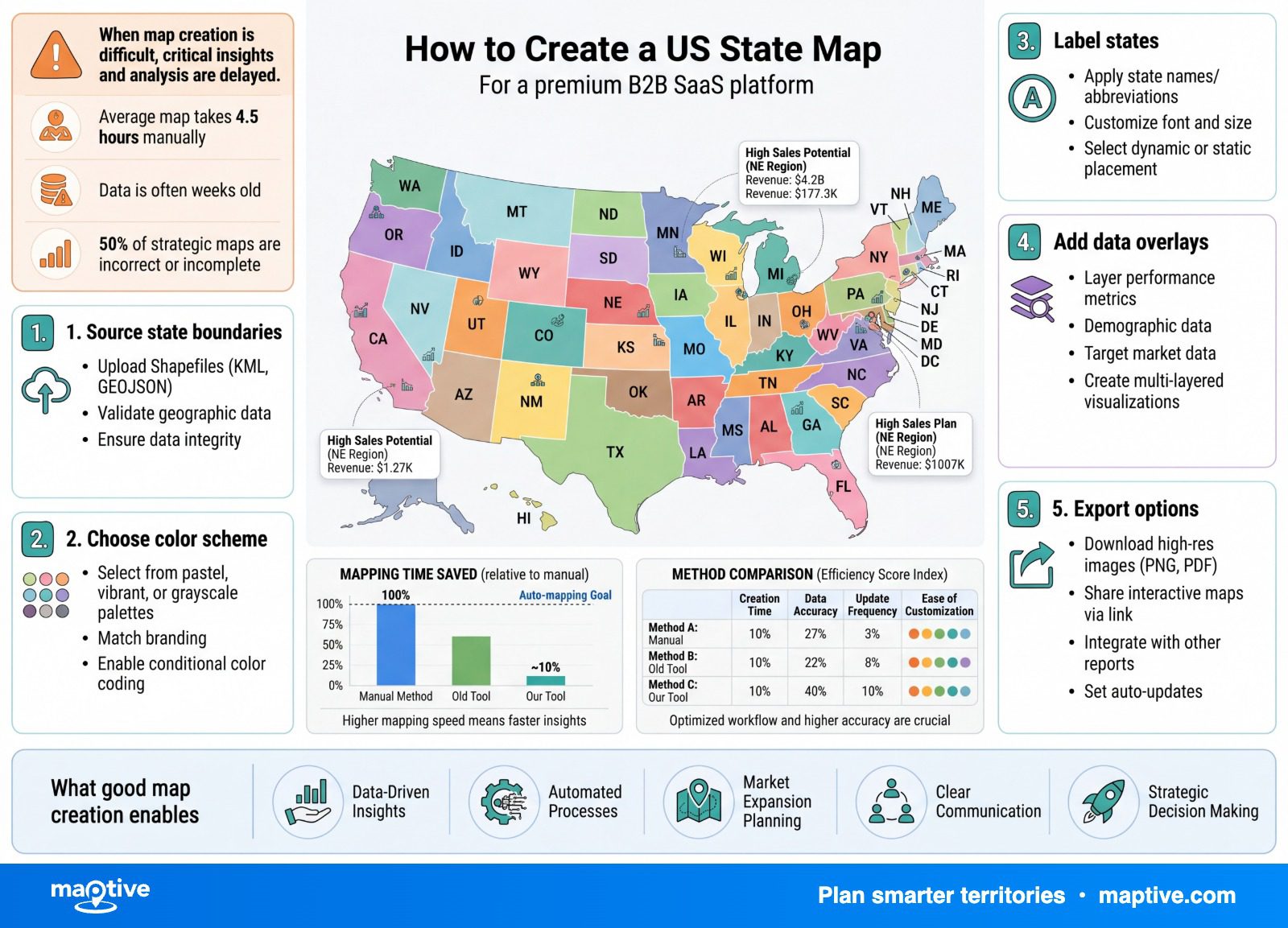
For the small northeastern states that cannot hold a name inside their borders, lean on two-letter abbreviations or a leader line out to a label, and on a data map let the value itself stand in as the label so you are not crowding all 50 names onto one screen.